The 41-Month Kitchin Cycle In Stocks │ Edward R. Dewey

Another cycle that has done all in its power to keep cycle scientists humble is one averaging 40.68 months in length. It has been present in industrial common-stock prices since 1871 and was discovered in 1912 by a New York group of investors. These gentlemen had learned that the Rothschilds had analyzed British consols (government obligations) and had broken up the price fluctuations into a series of repeating curves that had been combined and used for forecasting. The New York group hired a mathematician to discover the secret formula of the Rothschilds, and working with the Dow-Jones Railroad Averages, he discovered a forty-one-month cycle, plus three others, which his employers used to help them invest in the market. Apparently they were very successful around World War I.

 

Figure 38: The 41-Month Rhythm in Stock Prices, 1868-1945.

 

Some ten years after the original discovery, Professor W. L. Crum, of Harvard, noted a cycle of "39, 40, or 41 months" in monthly commercial-paper rates in New York. Almost simultaneously, Professor Joseph Kitchin, also of Harvard, discovered a cycle that he called forty months in six economic time series, bank clearings, commodity prices, and interest rates in both Great Britain and the United States from 1890 to 1922. As far as I know, it was not until 1935, twenty-three years after the original discovery, that this cycle was again noticed in the stock market. Our old friend Chapin Hoskins, who knew nothing of the earlier work, discovered this cycle in many series of price and production figures, including common-stock prices. Early in 1938 he made an extensive study of this cycle for one of the large investment-trust services.

Figure 38 shows the forty-one-month cycle (now refined to 40.68 months) from 1868 through 1945. As you can see, while its waves are not identical to an ideal 40.68 wave, which is represented by the broken zigzag, there is an amazing correspondence between them. This cycle persisted through wars and peace, good times and depressions.

Then, in 1946, something strange happened to our cycle. Almost as if some giant hand had reached down and pushed it, the cycle stumbled, and by the time it had regained its equilibrium it was marching completely out of step from the ideal cadence it had maintained for so many years. As you can see in Figure 39, it has regained the approximate beat of forty-one months or so, as before, but its behavior now appears upside down on our graph.

 

Figure 39: The 41-Month Rhythm, Upside Down, 1946-1957.

 

Scores of explanations and reams of paper have been expended to explain this behavior. We are familiar with most of the possibilities, such as distortion by random behavior, two or more other cycles of near lengths, and even a general public knowledge of this particular cycle, which may have had a distorting effect on its timing. But, in truth, no one can positively explain what happened in 1946 any more than they can explain the regularity of the rhythm for all the years that preceded it.

Quoted from:
Edward R. Dewey & Og Mandino (1971) - Cycles: The Mysterious Forces that Trigger Events.

 

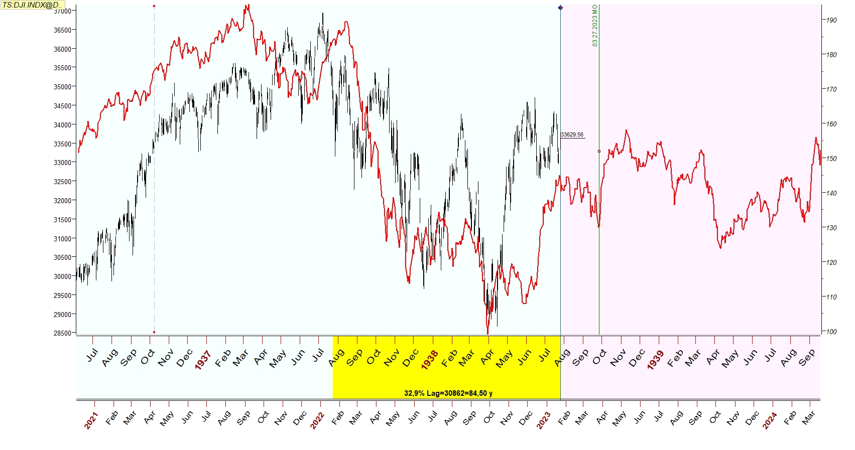
42-Month Cycle in the DJIA (weekly bars), March 2020 - October 2023.

S&P 500 Projection Into June 2024 | Allen Reminick

 

 

The November rally is likely to experience some downside pressure in the first half of December and the first half of January. 

After that, we expect higher prices until March and April of next year.

Quoted from:
Allen Reminick (Nov 18, 2023) - Market UP till April, But Watch for Down Moves. (video) 

 

The Art of Forecasting Wheat Prices Using Harmonic Cycles | L.H. Weston

Numerous attempts have been made during the past century to find a fairly reliable method for determining, long in advance, the probable price of wheat and grain in general [...] We have a wheat record that runs back, upon unimpeachable authority, for several hundred years, the one given in this booklet beginning in the year 1270 and running up to present time, with years as the unit of time, and it would indeed be strange if, with such a record, we could not pick out the useful cycles in it, providing any such cycles really do exist [...] That there are recurring cycles of movement in nearly all, if not, indeed, absolutely all natural phenomena, there is now no longer any reasonable doubt. No scholar of the day, no scientist, no investigator of these times, would for a moment argue against this well established fact.

 

[...] In the following pages I give the recorded mean price of wheat for each year in England from the year 1270 to 1909, in both a table and a diagram. Also, in a diagram, the monthly mean price of wheat at Chicago and Cincinnati from 1844 to present date. Special charts are also given to illustrate the explanations regarding the method of forecasting by means of cycles. By means of these tables and charts I show in this work how a forecast of the wheat market can be made up for over 40 years. In fact, I chart the forecast in advance over 10 years, for the benefit of readers and students. It is done just as proposed above, namely, by first proving that the harmonic cycles really do exist in the records, and then carrying them on into future years. The calendar year is used as the unit of time (or the calendar month) and therefore the forecasting, as taught, is necessarily of the long swing movement. 

 

 

 

[...] On page 27 is given the table of composite and harmonic values in the 49-year cycle. That composite is, as before stated, the result of eleven cycles added together, while the harmonic values are merely the smoothed curve of this same composite, and both are charted together on page 26. 

 

[...] This result is given in the Composite Chart of the 49-year cycle and it is the one used as the basis of all forecasting. If we examine the composite chart with some attention we will find that there are just about eight places where tops come out and likewise there are eight bottoms. Eight into 49 goes 6.125 times, so it seems very much as though the famous 7-year cycle of the ancient Jews was in reality about six and one-eighth years instead of 7. It is the eighth harmonic that gives the best results in the 49-year cycle, instead of the seventh.

Quoted from:
L.H. Weston (1923) - The Art of Forecasting Wheat Prices by the Use of Harmonic Cycles.

 

See also:
Hans Hannula (1993) - Gann's Greatest Secret: L.H. Weston - Gann’s Professor.
L.H. Weston (1921 & 1923) - Being a Treatise on the Geometrical or Chart System of Forecasting in which is explained the principles of the art, and, in this lesson no. 1, giving demonstration with the price curve of potatoes in the U.S.  

S&P 500 Cycles Forecast | Sergey Ivanov

S&P 500 / ES Major High = ± Sep 08-11, 2023 (Fri-Mon)

 

 

The 2nd half of this week [Sep 04-08] is going to be bullish for the index. Talking about the most probable date for expected (at daily time frame) bearish turn we may rely on the Moon cycle at M30 chart. If today's drop is considerable then a local top is was already set. The next date for local high will be reached by the end of Friday [Sep 08] or the very beginning of the next Monday [Sep 11].

Reference:
Sergey Ivanov (Sep 02, Sep 04 & Sep 05, 2023) - Forecasts calculated with Timing Solution software; published on Telegram.

Dow Jones Industrial Average Self-Similarity Charts for 2023 | Sergey Ivanov

1938 vs 2023

Highest Similarity Ratio between 1963 and 2023 - Projected Low of the Year is February 22 (Wed)

1966 vs 2023

1973 vs 2023

1982 vs 2023

2003 vs 2023

2009 vs 2023

Source:

Sergey Ivanov (Jan 24, 2023) via his free Timing Solution Forecasts Telegram Channel. 

See also:

Sergey Tarassov (2003) - Back Testing of Similarity Module.

Sergey Tarassov - Timing Solution Software.

Sergey Tarassov - Timing Solution Community Group.

Bearish Forecast for US Stocks Indexes | Sergey Ivanov

Sergey Ivanov (Nov 30, 2022) - We have two kind of very effective projection lines for the indexes: Self-Similarity vs 2008 year and Fixed Cycles Composite Line. As you can see they suggest an extreme bearish scenario for the next 1.5 months. If it already started or we have some additional expected bullish bounces is answered by temporal cycles projection lines. 

 

 

Source:
Sergey Ivanov (Nov 30, 2022) via his free Timing Solution Forecasts Telegram Channel  

See also:

Sergey Tarassov - Timing Solution Software

Sergey Tarassov - Timing Solution Community Group

The Name of God & The Rule of Nine | Martin A. Armstrong

Martin A. Armstrong (2008) - Just about everyone knows the "666" omen, but strikingly, most do not know the number of the name the Jews gave to God - "Jehovah." If we use the old Hebrew system we can find the number of God. Yod = 10, He = 5, and Van = 6. Therefore, the name of God in Hebrew He Van He Yod equals 5 + 6 + 5 + 10 = 26. The number of the name assigned to God by the Jews is 26.

 

 

I explained that I discovered the 8.6 year cycle by adding up the total number of financial panics between 1683 and 1907, which created a time-space of 224 years. I found that there were 26 financial panics and then divided that into the 224 years to obtain an average. That produced the 8.6 year frequency. Only when it began to project to specific days, then I decided to study much deeper. There is, the fact that it appeared to be intricately complex running concurrent with countless other cyclical behavior be it natural or man himself in a sort of time-space tube created by an interdependent, self-referral field network whereby, the output of each and every iteration becomes the input for the next generation perpetuating patterns of order in such a dynamic structure, that one cannot see the order of the whole for the mask of superficial chaos. There simply is yet a separate and distinct core frequency of 26 running through the center of the field causing not merely Phase-Transitions, but also Phase-Shifts and Phase-Cancellations when two cycles indeed collide of equal yet opposite forces.

1929 - 1955 - 1981 - 2007

The above sequence of dates provides a simple demonstration of the interesting relationship of 26 to the Economic Confidence Model. The high on the last Private 51.6 year Wave was 1929.75. If we simply take the annual count of 26, we produce the above time series, The great expansion of U.S. debt began from the 1955 post-war target where spending without regard to maintaining the ratio to gold may safely be defined as the start of the perpetual. spending. The next target 1981, was the high of the Public Wave of 51.6 years marked by the peak in interest rates and the open battle against inflation. This brings us to 2007, where the model has correctly given the high 2007.15 that targeted to the day, the start of this economic decline.

Previously, we looked at two time series, one beginning from 1775 marking the start of the American Revolution, contrasted with 1788 that marked the beginning of the federal government with the Constitution. The differential between these two series is half the 26 cycle - 13 years. It is twice 26 that produces the number 52 that we will see is central to the Maya, but was also the observation of the commodity cycle noted by Kondratieff - the Russian economist. We can see that the timing interval of 26 is a critical and interesting number to say the least.

 

Another kabala number of mystery has been attributed to the famous Gaon from Vilna who discovered that the Hebrew
word for truth (taf-mem-aleph) produces the number taf = 400, mem = 40, and aleph = 1 added together 441 = 9.
It was argued that God created the world based upon truth, which is the number 9. If you take any number greater
than 9, add the individual numbers, and subtract the original, we end up with a number divisible by 9.

 

Whether 26 is the "God Cycle" is interesting. Hipparchus of Rhodes observed around 150 BC that the equinoxes moved with time. This is where the Sun's path crosses the celestial equator. He realized that these were not fixed in time and space but traveled in a cyclical manner. The movement was extremely slow in a westerly direction. This amounted to but less than 2° in about 150 years. This slow movement is known as the "Precession of the Equinoxes" and requires generations to even observe. It is less than 2° movement every 150 years, bringing this also to a virtual number of close to 26,000 years to complete one cycle.

Quoted from:
Martin A. Armstrong (2008) - It's just Time

 

See also:
Martin A. Armstrong (1979) - The Fractal Design of Time
Martin A. Armstrong (2008) - The 8.6 Year Global Business Cycle 2002 - 2028

Martin A. Armstrong (2022) - ArmstrongEconomics - researching the past to predict the future

 

Periods When to Make Money | Benner Cycle Projection into 2023 Major Low

Samuel Benner was a prosperous American farmer wiped out financially by the 1873 panic and a hog cholera epidemic. In retirement, he set about to establish the causes and timing of fluctuations in the economy. 

 

Edward R. Dewey (1967):
» If you had used these dates for trading, your percentage gains between 1872 and 1939
would have been 50 times your losses! «

In 1875 he published a book called "Benner's prophecies of future ups and downs in prices" forecasting commodity prices for the period 1876 to 1904. Many - not all - of these forecasts were fairly accurate. The Benner Cycle includes:

• A (upper line): "Years in which Panics have occurred and will occur again." A 54 year cycle alternating every 18, 20 and 16 years.
  
• B (middle line): "Years of Good Times, High Prices and the time to sell Stocks and values of all kinds." Cycles alternating every 8, 9 and 10 years.
• C (lower line): "Years of Hard Times, Low Prices, and a good time to buy Stocks, 'Corner Lots', Goods, etc, and hold till the 'Boom' reaches the years of good times; then unload". A 27 year cycle in pig iron prices with lows every 7, 11, 9 years and peaks in the order 8, 9, 10 years (B - middle line).

Benner's cycle projections align with the latest analysis of the "Foundation for the Study of Cycles" and are pointing to a major stock market low in the US in 2023. David Hickson's Hurst cycle analysis projects this low to March of 2023 and Martin Armstrong to April 11, 2023 (Tue).

 

» Periods When to Make Money « ; the original business card of George Tritch Hardware Co.
Apparently, the diagram was compiled by George Tritch in 1872, but was not attributed to
him by Samuel Benner in 1875.

 

References:

 George Tritch (1872) - "Periods When to Make Money" - Business Card of George Tritch Hardware Co.

Samuel Benner (1884) - Benner's prophecies of future ups and downs in prices (3rd. Ed.; original 1875)

 W.D. Gann (1909) - Financial Time Table 1784 - 2102

Edward R. Dewey (1967) - The Case for Cycles 

Elwynn Taylor (2004) - Crop Weather Cycles: Myth or Reality?

Martin A. Armstrong (2008) - The 8.6 Year Global Business Cycle 2002 - 2028

Charles Capriole (2020) - George Tritch Strategy from 1872 has a 90% hit rate
David McMinn (2022) - Benner Cycles & the 9/56 year grid

David Hickson (Oct 3, 2022) - The Next 20 Weeks - S&P 500 - Hurst Cycles Market Update
Lars von  Thienen (Oct 9, 2022) - Market Cycles Report - Cycles of Financial Crisis using long term static cycle models.

TPR (2015) - Future Ups and Downs into 2065. Samuel Benner’s Prophecies.

 

The Tritch / Benner Strategy yielded 7,939% from 1872 to 2020

George Marechal's Stock Market Forecast 1933 to 1948 │ Law of the Market

In 1933 the incoming U.S. President Franklin D. Roosevelt reached out to Roger Ward Babson for a long range forecast for the stock markets. Babson, a very successful entrepreneur, economist, business theorist, investor, and philantroph with a huge fortune, was a household name since he had predicted, back on September 5th 1929, that "a crash is coming, and it may be terrific". Later that very same day the stock market on Wall Street declined by 3% and this became known as the "Babson Break". The big crash with most catastrophic losses followed on October 24 and 29, 1929 (Black Thursday and Black Tuesday). When the U.S. finally reached the height of the Great Depression in 1932 and the stock market was at an all-time low, 75% of its value was wiped out, and shares in any company were virtually worthless. Thousands of people were ruined, and soup kitchens sprang up on street corners as people lost their jobs, savings and homes. 

To comply with President Roosevelt’s demand, Babson in turn consulted the largely unknown Canadian mathematician George Marechal, who recently had managed to work out how the highs and lows of the Dow Jones Industrial Index repeated themselves in predetermined sequences. So finally it was Marechal who produced a Dow Jones Index Forecast Chart over the next 15 years for the Roosevelt administration, that proved to be spectacularly accurate. So confident was Marechal in his prediction at the time that he had his chart copyrighted. His friend Alan H. Andrews (the inventor of Andrews’ Pitchfork) described it as a "chart no government economist, no college professor has enough knowledge to even approach or courage to try to duplicate." 

Comparison of Marechal's 1933 forecast with actual data of the Dow Jones Index from 1934 through April 1951
[published by Garfield A. Drew and Edward R. Dewey in Cycles Magazine, October 1962].

Edward R. Dewey confirmed in 1962 that still little to nothing was known of Marechal's method, though a fund manager had offered him $20,000 for his secrets, or, alternatively, to operate a five million dollar fund on the basis of these secrets and to share profits. But Marechal did not accept either offer, and finally died at the age of 90 without ever revealing how he was able to calculate market movements with such uncanny accuracy. However, what is clear is that he was using a version of Babson's Normal Line. The annotations to his chart later added by his friend Alan Andrews show that Marechal plotted turns with what are now known as Median Lines. Dewey concluded:

"The important thing about this study [chart of Marechal] is not the exact precision by which it came true, or the amount of money you would or would not have made if you had followed it. The important thing is that it shows that the market has predictable patterns. In other words, that the seeming disorder of market fluctuations really is subject to law, and that this law is learnable."

In 1948 Garfield A. Drew, another friend of Marechal, reproduced the forecast in his book "New Methods For Profit in the Stock Market". Drew stated that one of the original copies of the forecast had been in his possession since 1935, and as each year was divided into six parts he added in his book the actual fluctuations of the Dow Jones Industrial Averages by plotting the high and low for each two-month period. Drew commented on the famous chart:

"Clearly, the pattern of the forecast and the actual pattern of the market miss many times in detail and exact timing. Nevertheless, the broad picture of the trends from 1934 through 1947, at least, is remarkably similar. The basic downtrend from 1936-37 to 1942 is plain, and likewise the uptrend from 1942 to 1946, although the latter shows up as a much more zigzag pattern in the forecast than was actually the case. Thus, the year 1944 by itself, for example, appears as a down period, whereas it was really an up year. When the year 1947 ended, the Dow Jones Industrial Average had spent 16 months within a 16% price range. As far as the situation at the time the comparison in [the figure] ends is concerned, it is evident that, if the broad accuracy of the preceding 14 years is to be maintained, 1948 must, on the whole, witness a rising price level. A definite down trend going substantially into new low territory by the year-end would produce a greater discrepancy between the forecast pattern and the actual course of prices than at any other time in the record. The fact remains to be seen at this writing, but, in line with his original forecast made years before, Marechal always insisted that 1946-47 was not a "bear market" but an interruption in a long upward trend comparable to the break and market hesitancy during 1926 in the long upswing from 1921 to 1929.”

"In this figure the Dow Jones Averages are plotted from 1897 through 1962. On this chart are a number
of "resistance" lines. The original worksheets for Marechal's forecast look just about like this chart,
except that there were a great many more lines and, thus, a great many more intersecting points.
Marechal's secrets consist fundamentally of how to draw the resistance lines and how to select the
significant intersections" [Edward R. Dewey in Cycles Magazine, October 1962].

Wheels Within Wheels | The Vedic Concept Of Time

"Outside of the three planetary systems, the four Yugas multiplied
by one thousand comprise one day on the planet of Brahma. A similar
period comprises a night of Brahma, in which the creator of the
universe goes to sleep."
Srimad Bhagavatam, Canto 3, Chapter 11, Text 22

The Vedas and the Puranas describe a number of time cycles within cycles, from Paramanu (about 17 microseconds) to Maha-Manvantara (311.04 trillion years). The creation and destruction of the universe is a cyclic process, which repeats itself forever. Each cycle starts with the birth and lifetime of the Universe equaling 311.04 trillion years, followed by its complete annihilation which also prevails for the same duration (HERE).  

The universe always existed. It was not created, and the concept of eternal and cyclical time lies at the heart of the Hindu philosophy. In the Hindu conception of time there is no final cataclysm. The closing of one door implies the opening of another. 

Michael A. Cremo (1996): "Linear-progressivist time concepts [...]
pose a substantial barrier to truly objective evaluation of the
archeological record and to rational theory- building in the
area of human origins and antiquity." (HERE+ HERE)

Destruction of the cosmos only portends its re-creation. The entire material world is thus subject to everlasting cycles of creation, sustenance and destruction. This idea is closely related to the concept of Atman (the eternal self), ever-existing, not only in the future but also from the past. This notion of two-way eternity, however, is not reserved solely for the realm of spirit (Brahman) but extends to this temporal world. This universe exists for the lifetime of Brahma, the creator. His one day is 1,000 Maha-Yugas (Great Ages). The Puranic concept of time involves cycles of Yugas (Ages), each progressively shorter and more degraded.  

Each Yuga cycle is composed of four Yugas. The first, Satya-Yuga, is the Golden age and lasts 1,728,000 years. The second is the Silver Age, the Treta-Yuga, which lasts 1,296,000 years. The third is the Bronze Age, the Dvapara-Yuga, which lasts for 864,000 years. And the fourth is the Iron Age, the Kali-Yuga, lasting for 432,000 years. This gives a total of 4.32 million years for the entire Maha-Yuga cycle, the period of a Great Year. 

One thousand of such cycles 4.32 billion years make up one Day of Brahma, the demigod who governs the universe. One Day of Brahma is called a Kalpa. Each of Brahma's Nights lasts as long as his day. Life is manifest on earth only during the day of Brahma. With the onset of Brahma's night, the entire universe is devastated and plunged into darkness. When another day of Brahma begins, life again becomes manifest. Each Day of Brahma is divided into 14 Manvantara periods, each lasting 71 Yuga cycles. Preceding the first and following each Manvantara period is a juncture (sandhya). Typically, each Manvantara period ends with a partial devastation. 

Today we are living in the 28th Yuga cycle of the 7th Manvantara period of the present Day of Brahma. This would give the inhabited earth an age of 2.3 billion years. Altogether, 453 Yuga cycles have elapsed since this Day of Brahma began. Each Yuga cycle involves a progression from a golden age of peace and spiritual progress to a final age of violence and spiritual degradation. At the end of each Kali-Yuga, the earth is practically depopulated.  

Currently, 50 years of Brahma have elapsed. The last kalpa at the end of 50th year is called padma kalpa. We are currently in the first 'day' of the 51st year. This Brahma's Day, Kalpa, is named as Shveta-Varaha Kalpa. Within this Day, 6 Manvantaras have already elapsed and this is the 7th Manvantara, named as – Vaivasvatha Manvantara. Within this Vaivasvatha Manvantara, 27 Maha-Yugas, and the Krita, Treta and Dwapara Yugas of the 28th Maha-Yuga have elapsed. 

The current Kali Yuga began at midnight of February 17th to February 18th in 3102 BCE in the proleptic Julian calendar. As per the information above about Yuga periods, only 5,118 years are passed out of 432,000 years of current Kali Yuga, and hence another 426,882 years are left to complete this 28th Kali Yuga of Vaivaswatha Manvantara.The time elapsed since the current Brahma has taken over the task of creation can be calculated as

432,000 × 10 × 1000 × 2 = 8.64 billion years (2 Kalpa - Day and Night)
8.64 × 109 × 30 × 12 = 3.1104 Trillion Years (1 Year of Brahma)
3.1104 × 1,012 × 50 = 155.52 Trillion years (50 Years of Brahma)
(6 × 71 × 4,320,000) + 7 × 1.728 × 10^6 = 1,852,416,000 years elapsed in the first six Manvataras, and Sandhi Kalas in the current Kalpa
27 × 4,320,000 = 116,640,000 years elapsed in first 27 Maha-Yugas of the current Manvantara
1.728 × 10^6 + 1.296 × 10^6 + 864,000 = 3,888,000 years elapsed in the current Mahayuga
3,102 + 2,016 = 5,118 years elapsed in the current Kali Yuga.

So the total time elapsed since current Brahma is: 155,520,000,000,000 + 1,852,416,000 + 116,640,000 + 3,888,000 + 5,115 = 155,521,972,949,117 years (one hundred fifty-five trillion, five hundred twenty-one billion, nine hundred seventy-two million, nine hundred forty-nine thousand, one hundred seventeen years) as of 2016 A.D.

The main time cycle governing mankind is the precessional cycle:
The period of 25,000 years the seasons in the life of humanity.

Surya Siddhanta: "A lunar month, of as many lunar days (tithi);
a solar (saura) month is determined by the entrance of the sun
into a sign of the zodiac; twelve months make a year. This is
called a day of the gods."

The Periodic Table of Commodity Returns

U.S. Global Investors (Jan 27, 2016) - This table shows the ebb and flow of commodity prices over the past decade.

The Fractal Design of Time | Martin A. Armstrong

 

 

The Economic Confidence Model (ECM) is a computer model that analyzes the global economy by tracking capital flows and concentration, providing a macro long-term perspective of when shifts in confidence are possible that could lead to notable economic events as demonstrated over the course of history.

• The model consists of cycle waves that vary in length, from shorter to longer, and build up over time; for example, 8.6 to 51.6 to 309.6 years.
• It examines these cycle waves to discover when they are set to culminate, reflecting a possible shift in market confidence at that point in time.
• This shift in confidence is reflected by capital flows and concentration.
• The longer the cycle wave, the greater the magnitude of the shift in confidence.
• The dates in the model that reflect possible shifts are referred to as ECM turning points.

The ECM does not track or forecast individual financial instruments, securities, or markets.

The Sun, the Moon, and the Number 56 | David McMinn

References:

Sunday, October 1, 2017