Thursday, March 21, 2024

The 500 Year Cycle | Raymond H. Wheeler

The 1000 year cycle tends to break down into halves of about 500 years each. Centering on the dates of 375 BC, 30 AD, 460 AD, 955 AD, and 1475 AD, climate was dry and colder than usual. The warm periods were short and were often disrupted by drops in temperature. Midway between these dates, the warm periods stretched out; the interruptions were not as long, and the cold periods shortened. The result is an intermediate cycle averaging 510 years in length.
 
 » Mass migrations were extensive, and all the ancient civilizations collapsed. «
Vandals sacking Rome, 455 AD.

The beginning of the first of these 500-year rhythms marks an important place in the history of climate. Prior to 575 BC, climatic cycles were longer and more extreme than they have been since then. In the two centuries immediately following, from 450 ta 320 BC, it was warm much of the time. Two 100-year cycles were almost fused into one. The cold period between them, at 420 BC, was very short. After that, the cold periods lengthened. By the end of this 500-year period, at the time of Christ, there was an exceptionally long cold period.

The cold phase centering on 460 AD, at the end of the next 500-year cycle, was also exceptionally cold. Mass migrations were extensive, and all the ancient civilizations collapsed. There was a long-term downward trend in rainfall. Although there were long cold phases in the 600s and 700s, they were frequently interrupted by silts to the warm side and did not seem to be exceptionally bad. The cold phases of the 800s and 900s were extremely severe, causing many migrations, primarily from the northern countries — especially when conditions began to deteriorate approaching 955, near the end of the 500-year rhythm.
 
 » Civilizations broke up and new ones took their places. «
 Migrants storming European Union borders, 2024 AD.

Subsequently, temperatures warmed suddenly. The 1000s were so warm that trees grew in Greenland. This was the period when Vikings crossed the Atlantic, One of the most severe hot droughts in history occurred in the 1130s. The 13th century saw a long warm period. Then climate began to deteriorate again. While the 14th century was warm much of the time, there were frequent and sharp drops in temperature; often it was very stormy. During several winters, the straits between Denmark and Sweden froze over solid enough to support horses and sleds, Greenland began to freeze. In the 15th century, there was no long warm period.

The next 500-year rhythm terminated at 1475. Subsequently, temperatures warmed up again. The 17th century was so warm that the next 100-year cycle had but a short cold phase, centering on 1655, and this was quickly interrupted by a shift back to the warm side. During the 19th and 20th centuries, climate deteriorated again.

 
» The 500 year period beginning at 1475 is drawing to a close. «
 Migrants breaching US southern border, 2024 AD.
Climate change? Sure.

Events of great importance occur every 500 years. Midway between 575 BC and 460 AD, the Roman Empire began its decline as Christianity rose. There were no strong European civilizations for a long time. On the other hand, there were very strong Asiatic empires such as that of the Huns. Midway between 460 and 1475, in the 9th and 10th centuries, a vast change occurred, again involving mass migrations, These events divided the Middle Ages into two halves. In the first half, there were brilliant empires like those of Justinian with its capital at Constantinople, Charlemagne in the West, and the Arabs in the East. The Arabs moved into Spain and India, developing brilliant civilizations at Cordoba and Bagdad. But all this came to an end. These civilizations broke up and new ones took their places. Following 975, the feudal period developed, with the growth of principalities that were to form modern European states. Amazing empires were built by the Mongols in Asia, the Incas in South America, and the Mayas in Central America. In India and Japan, new empires were born. The Balkans achieved their Golden Ages during this period.

All this came to an end in the 15th century. The Medieval economy, customs, and modes of thought disappeared. With the new 500-year climatic cycle came the Renaissance, the Reformation, and the building of modern nations — first under absolute monarchs, then under constitutional governments. This most recent 500-year cycle has witnessed the awakening of modern art, science, and economics. In these more advanced civilizations, the common people have, for the first time in history, come into their own under democratic political and economic systems.

 » The same types of events occurr with almost clock-like regularity. «

The 500 year period beginning at 1475 is drawing to a close. We are now witnessing many of the same types of events that have occurred under similar circumstances with almost clock-like regularity five times before in history. These events are of the utmost significance for the businessman and student of today — and tomorrow.
 
Quoted from:
Raymond H. Wheeler (1943) - The 500 Year Cycle. 
With a Forecast of Trends Into the 21st Century.
 
  » A 500-year cycle is now terminating, which belonged to Europe.
The next 500-year cycle will belong to Asia.
«
Raymond H. Wheeler, 1951.

See also:
Raymond H. Wheeler (1943) - The 100 Year Cycle - Climate, Regime Change and War.
Donald A. Bradley (1943) - Cycles Write World History.

Sunspots, Lunar Cycles and Weather Cycles | Louis M. Thompson

The occurrence of an 18- to 20-year cycle in weather in the U.S. Midwest is no longer controversial. The controversial issue is the cause. This article will present both sides of the issue, and will indicate why we will know more about the cause after the 1990s.


[...] The sunspot cycle has been associated with the “20-year drought cycle” in the western U.S. since about 1909, when A.E. Douglass started publishing his tree-ring studies. This scientist became so well known that he was able to establish the Laboratory for Tree Ring Research in Tuscon, Arizona, in 1938. 
 

[...] The sunspot cycle has averaged about 11 years since 1800. As the sun rotates on its axis, it makes a complete turn in about 27 days. Large and persistent spots appear to move from left to right for about two weeks, disappear, and return after about two weeks. The leading edges of spots or clusters of spots have a negative charge in one 11-year cycle and a positive charge in the next cycle. Hence, the term “double sunspot cycle.”


The conventional wisdom is that the drought cycle of about 20 years occurs near the end of the negative cycle and at the time of low solar activity. The drought periods of the 1910s, 1930s, 1950s, and 1970s occurred at the end of the negative cycle. The drought periods did not consistently follow that pattern from 1800 to 1900, although the severe droughts of the 1820s and 1840s occurred at the end of the negative cycle.

Quoted from:
Louis M. Thompson (1989) - Sunspots and Lunar Cycles: Their Possible Relation to Weather Cycles.
In: Cycles, September/October 1989, Foundation for the Study of Cycles.
 
See also:
William Stanley Jevons (1875) - Sunspots and the Price of Corn and Wheat.

The 18.6 Year Cycle in the General Economy | Louis M. Thompson

I believe there are weather cycles that trigger events in our economy, and I believe there is one weather cycle that is related to the 18.6 year lunar cycle. For that reason, I have prepared a lunar declination chart patterned after Fig. 1 and shown as Fig. 3. If a relationship between the lunar cycle and the weather cycle can be explained, we will gain a real milestone in explaining the business cycle.


[...] We have a 9.3-year cycle in production, which gives rise to a 9.3-year cycle in grain prices. Highest yields have occurred at the time of minimum declination and the four following years. Lowest prices have occurred because of a build-up of supplies, and the low prices have occurred about every 9.3 years and every 18.6 years. Fig. 3 describes the cycle in agriculture better than it does the general economy. Yet, as we look back to the nineteenth century, there were depressions at the time of maximum declination (285°) in every 18.6-year cycle. In this century, our lowest agricultural prices occurred in 1913, 1932, 1950, 1969, and 1987, or every 18.6 years. lt appears that a weather cycle of 18.6 years drives a production cycle of the same length, which drives a price cycle of the same length.

Quoted from:
Louis M. Thompson (1989) - The 18.6-Year Cycle in the General Economy.
In: Cycles, May/June 1989, Foundation for the Study of Cycles.
 
See also:
In: Cycles: The Science of Prediction.

Predictable Cycles in Geomagnetic Activity | Theodor Landscheidt

Geomagnetic storms, which are released by energetic solar eruptions, are important geophysical events. Newer results indicate that there is a connection with weather. Figure 1 shows the zonal type of atmospheric circulation as a result of geomagnetic disturbances caused by the sun’s eruptional activity, and meridional circulation related to a lull in geomagnetic activity. This is a permanent feature that regulates the prevalence of warm westerly flow or cool arctic air over Europe and North America. 


The bulk flow speed of the solar wind, which is indicative of the energy of eruptional mass ejections and resultant shock waves caused by solar eruptions, is strongly coupled to geomagnetic activity, which in turn seems to be the common factor of a wide variety of terrestrial phenomena.

Quoted from:
Theodor Landscheidt (1989) - Predictable Cycles in Geomagnetic Activity and Ozone Levels.
In: Cycles, November/December 1989, Foundation for the Study of Cycles.

Tuesday, March 19, 2024

Election Years Are Different | Tom McClellan

I have been writing about the Presidential Cycle Pattern since 1994, using the pattern which is derived from averaging together SP500 price data in 4-year chunks of time. One difference in how I do this versus others is that I start each 4-year period as of November 1 instead of January 1, to better align with election day. This week's chart looks at the differences (and similarities) in the versions of the Presidential Cycle Pattern depending on what type of president is in office. The green line reflects first term presidents from a different party than the last president, and reflects the condition we have now.

  » March is typically a sideways month, part of a larger sideways pattern 
lasting all the way until late May. The market normally rallies from June to election day. «

[...] A lot of the time, the two patterns behave very similarly. But in March of the election year, there is a notable difference. When a first term president is in office and running for reelection, March is typically a sideways month, part of a larger sideways pattern lasting all the way until late May. March is different, though, when a second term president is in office (red line). [...] The stock market normally rallies from June all the way to election day
[November 5] when there is an incumbent running for reelection. And usually an incumbent will win reelection. That is how things normally go.
 
Larry Williams identified June 2024 in the current decennial pattern
 as  » the sweet spot with 90% accuracy « to buy and hold until December 2025

[...] This year we have a challenger who is not an unknown quantity (to Wall Street), who at the moment has a slight lead in the polls. This type of condition is totally backwards from how election years usually go.  Add to that the additional unknowns about how President Trump is facing multiple trials for alleged crimes, and we have an election year completely unlike any previous one.  So trying to run a forecast model based on how things have gone in prior election years may just not work this year.
 

Monday, March 18, 2024

ICT Liquidity Runs | Michael J. Huddleston

As price action traders, we're looking specifically for reference points where there is a high probability of liquidity resting in the marketplace. Related to ICT concepts, liquidity relates to buy orders and sell orders. It's as simple as that.

Below old lows, the market will seek liquidity for the sell side or the sell stops, taking orders out. Understanding this premise, when we view price action, it removes all of the retail-minded perspective but heavily leaning on indicator-based ideas. When we adopt these principles with study of price, it gives us the  truest and purest view of how price is delivered.

We have no confidence or direct relationship to our directional bias on price relative to anything except for price itself. If the market is moving from an old high, we know that there is going to be liquidity resting above that old high. If the market is moving from an old low, we know there is going to be a rest liquidity below those lows. It is just that simple. 
 
LRLR = Low Resistance Liquidity Run
HRLR = High Resistance Liquidity Run

As a trader you want to be trading when there is LRLR conditions because during LRLR conditions price will cleanly deliver to your target a lot quicker than HRLR conditions. If you're in a trade a lot longer than expected it is most likely because you are in HRLR conditions.

A LRLR will have clean highs or lows and for this example it means there's a large pool of liquidity resting above the Clean Highs/EQHs. This is where retail traders are placing their stops and smart money will look to take out these stops.


Another way you can look at LRLR is if there are EQH/Ls & multiple highs/lows lined up in a row (Trendline Liquidity). This is what #TheStrat traders call Pivot Machine Gun (PMG). It's called PMG because the algorithm spools higher like a machine gun triggering stop losses to get taken out.


So in this example, after SSL got raided, you're looking to go long inside of the FVG within the BPR to target the EQH. This is LRLR conditions.


When you have EQH/L, any PD arrays in-between where price is currently at to the EQH/L will have a low probability of holding. Smart money will target the largest liquidity pool which will be the EQH/EQL so price will either go through the PD array, or consolidate at the PD array then continue in the direction of the EQH/L. Now we will look at an example of HRLR. Typically with HRLR conditions there will be a stop hunt (fu) on buyside or sellside liquidity. Once there's a stop hunt it will leave a Point of Interest (POI) / PD array which is typically an orderblock or fair value gap.


Because there's a stop hunt (fu) which leaves a POI, the POI will act as resistance which will make it a HRLR condition. So in this example, instead of going long at the lows to target the high formed from (fu), I'd rather wait for price to reject off the POI to look for shorts.
 

1st pic below is M15 timeframe, 2nd pic below is H1 timeframe. You will see a M15 fu raid on BSL which leaves an H1 bearish orderblock making it HRLR. After the fu raid price went lower and when it retraced back up it rejected the orderblock then started to take out internal SSL.


HRLR conditions can also happen when indices ( $ES $NQ $YM ) is not in sync with each other or when it's not in moving inversely to $DXY (dollar). $GU & $EU are supposed to move inversely w/ $DXY as well so if they're moving together it is HRLR conditions.


Reference:
 

ICT Draw on Liquidity | Darya Filipenka

Liquidity is the lifeblood of the markets. Liquidity is what allows anyone to buy or sell for a profit or a loss. It is what creates opportunity in the markets. While liquidity may not hold much significance for a retail trader, it is of paramount importance to big players who must carefully consider it in order to execute positions successfully. In an non-liquid market there are few buyers and sellers, and trades may take longer to complete, and prices can be more volatile. To help you better understand what liquidity is, I have drawn some simple diagram. It illustrates why we refer to certain levels as 'liquidity'. The point is not that the models themselves are liquidity, but that when a certain price model appears, liquidity is attracted at key levels and price points.


So what is the use of liquidity for us traders? Good question. Liquidity helps us determine where the price is likely to go next. You can learn to trade only using liquidity levels, it's not difficult, but the risks and potential profits will not be so attractive. In order to get a high-quality trading idea, using the liquidity, you need to apply the market structure on the Higher Time Frames, order blocks, and Premium/Discount zones. This helps to understand what kind of liquidity will attract the price and where we should enter into the trade and where we should exit.

How to identify the Draw on Liquidity (DOL)? As a day trader, the DOL can be PWH/PWL (Previous Week High/Low), PDH/L (Previous Day High/Low), or session High/Low from Asia, London, or New York paired with EQH/EQL (Equal Highs/Lows) with a Low Resistance Liquidity Run (LRLR) condition. EQH/EQL (Equal Highs/Lows) are large pools of liquidity so institutions will always draw towards those levels to take out retail.

How do I find the next Draw on Liquidity? First thing, price is always either re-balancing or taking liquidity. Price is going from Premium/Discount array to P/D array. Hence, you must annotate your P/D zones to know If price re-balanced or will re-balance, you must also annotate your liquidity and P/D arrays. To find the next draw on liquidity, you can follow a displacement, use the reaction on a P/D array.

External range liquidity refers to the buy side liquidity above the range high and sell side liquidity below the range low in the current trading range. It Is associated with liquidity runs that seek to pair orders with pending order liquidity, which is in the form of a liquidity pool. External range liquidity runs can be low resistance or high resistance in nature. As a trader, you want your trades to be In low resistance conditions, meaning you don't want any resistance in your path of profitability. While Internal Range Liquidity is the liquidity inside the defined range (External Range Liquidity), This could be In form of any institutional reference that we can use as entry such as order blocks, fair value gaps, volume imbalance, and more.
 

ICT Algorithmic Price Delivery & Time Macros Intro | Darya Filipenka

Algorithmic macros are short lists of directives that trading algorithms follow to seek out liquidity and inefficiencies in the market. These macros are like a fishing rod, casting out into the market to identify and capture opportunities. These price action segments typically occur in 20 minute intervals. They involve a set of instructions that algorithms use to search for liquidity or market inefficiencies. They focus mainly on the first 20, 30, or 40 minutes of the trading hour, which starts at 9:30 EST/EDT.


The macro between 9:50 and 10:10 am is a time window where the algorithm starts its run for liquidity. One important aspect to note is the role of macros or specific time windows in the market. These macros provide us with valuable insights into when the market is likely to exhibit certain behaviors, such as running for liquidity or inefficiency.

The period between 10:50 am and 11:10 am marks the end of the 10:00 am to 11:00 em hour, which ls the first 90 minutes of trading. This transition from the morning session to the New York lunch period often leads to consolidation or a reversal in the market. Traders can anticipate this consolidation of reversal and adjust their trading strategies accordingly.

To effectively utilize algorithmic macros, traders need to analyze the daily chart and identify key levels (Order Block (OB), Breaker Block (BB), Fair Value Gap (FVG), etc.). In the given context, the ICT mentions a daily bullish order block. This order block consists of the high, the wick, and the opening of the daily propulsion block. Additionally, the ICT highlights the importance of fair value gaps within order blocks. These gaps represent areas of inefficiency or liquidity in the market.

In the world of trading. there are certain events that have a significant impact on market performance. One such event is the non-farm Payroll release. This event, which occurs on a monthly basic, provides crucial data on the number of jobs added or lost in the United States, excluding the farming industry. The non-farm payroll release is closely watched by traders and investors as it provides insights into the strength of the economy and can potentially move the markets. When the data is released, it often triggers orally or a decline in prices, depending on whether the numbers are better or worse than expected. During a non-farm payroll event, we can observe & specific pattern in price action. The market typically experiences sn initial rally, followed by s retracement or a drop to take out stops. This retracement is a strategic move to shake out traders who entered the market based on the initial rally. After the retracement, the market often resumes its upward trajectory.

 
Reference: 

Saturday, March 16, 2024

Sun - Earth - Man | Theodor Landscheidt

The unanimous message of mystics of all ages that all entities in the universe are interconnected and constitute an indivisible whole is proven now by unequivocal physical experiments that have been replicated again and again. From this undeniable unity, connectedness, and inseparability follows that any action or configuration in any distant part of the universe can influence processes in the Solar System inhabited by Man. This is also valid for the interrelations of Sun and planets within the Solar System and especially the Earth's connections with other cosmic bodies in the solar environment.

 » The whole of space is filled with electrons and flying electric ions of all kinds. 
We have assumed that each stellar system in evolution throws off electric corpuscles into space. 
It does not seem unreasonable therefore to think that the greater part of the material 
masses in the universe is found, not in the solar systems or nebulae, but in 'empty' space. «
Kristian Birkeland, 1913.

To look at the solar system and its constituent parts as a whole that embraces a complex web of holistic interrelations, is a premise of traditional astrology, which seemed antiquated, but turns out to be trend-setting. Thus, it appears promising to subject the astrological thesis of an influence of celestial bodies on the Earth and life on its surface to a new test. The quality of the astrological body of theses matches the holistic results of modern research, as it represents the archetype of an integrating science. Astrology of this brand was a historical reality in the era of Kepler, Galileo and Newton. It is well known that Kepler was both an astrologer and one of the creative founders of modern science. Book IV of his principle work Harmonices Mundi (1619) with the heading Book on Metaphysics, Psychology, and Astrology is evidence of this, as well as his papers De fundamentis astrologiae certioribus (1602) and De stella nova (1604). Those who pretend that Kepler was not really engaged in astrology should read these writings.

Friday, March 15, 2024

S&P 500 Index vs 18.61 Year Lunar Node Cycle │ March - April 2024

 
» I’m not trying to predict the future; I am trying to accurately and quickly depict the present. 
I’m not trying to predict what people will do, but rather identify what they are doing right now. «  
Chris Camillo, 2023
 

Thursday, March 14, 2024

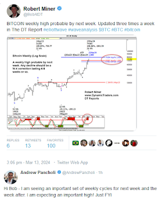
Bitcoin weekly high probable by next week | Robert Miner

Any decline should be lasting 6-8 weeks.
 

Happy Pi Day | Martin A. Armstrong

Perhaps it was my fate or destiny since I grew up in Maple Shade, New Jersey, with the house address of 314 South Lippincott Avenue. What a coincidence.


When I discovered that list of international panics and divided simply 26 into 224 years, it came out with 8.6153. Multiply that by 365 days = 3,144. Suddenly, the accuracy of the Economic Confidence Model (ECM) made sense – it was Pi, the magic number that the Egyptians even used to build the Pyramids.
 
 
See also:
 
 [The ECM does not track or forecast individual financial instruments, securities, or markets.]

A Lunar Chaos Theory | Al Larson

As the planets orbit the sun, they exert tidal forces upon the gases of the gun, much as the moon raises tides on the earth. The equation below describes these forces. Numerical solution of this equation reveals that Jupiter, Mercury, Venus, Earth, Mars, and Saturn are the most Influential, in that order. In Figure 1 shows this tidal effect caused by planets 1 and 2 rotating a gaseous portion of the sun's surface. These gas swirls cause several solar effects, including sun spots, coronal holes, and solar flares. All these effects combine to vary the amount of radiation that leaves the sun.
 

This solar radiation travels toward the earth in two ways, as direct radiation, such as sunshine and radio waves, and as particles, carried by the solar wind. This flow of charged particles forms a torrent of energy that blast spaceship earth, creating a bow wave and a wake just as a boat going upstream would do. This bow shock wave forms a magneto-pause between the earth and the sun. It interacts with the earth's magnetic field, shaping and adding energy to it. At the north and south poles, the charged particles follow the magnetic lines of force, and enter our atmosphere in a Polar Cap Absorption Event. This leads to the auroral oval, producing our Northern and Southern Lights.

The bow wave also creates an envelope about the earth, called the magnetosphere. As the solar wind flows past the earth, the magnetosphere forms a teardrop shaped envelope of trapped particles, ending in the magneto-tail. It is inside this envelope that the moon orbits. As the solar radiation varies, so does the earth's magnetic field, atmospheric ionization, and temperature. Scientists have tracked down a host of relationships between these events and a variety of earthly phenomena such as climate, weather, crime rates, plant growth rates, frequency of thunderstorms, blood PH levels, psychiatric emergencies, etc.  My own work has related these events to market action as well.


I believe there is also a third mechanism at work, one involving the moon. Let me explain: The moon's orbit is the most complex of all the ten bodies under consideration. While a planet's position may be accurately computed from an equation containing about nine or so terms, computing the moon's location to the same accuracy requires over 100 terms. Some of these terms are directly traceable to the pull of various planets and the sun on the moon. For example, there is a term related to Venus, our closest planetary neighbor. All these terms still do not describe a stable orbit, but one that rotates slowly In space, coming back to the same orientation in about 18.6 years. This is the moon's nodal cycle. Most people are familiar with the moon's full moon, new moon, or synodic cycle of 29.531 days. Many have tried to correlate it with market movements. The moon has many other cycles. It moves closer to and further from the earth, in what is the moon’s anomalistic cycle, which ls 27.554 days long. As the moon passes through the ecliptic plane (the plane of the earth's orbit) it crosses at its node, to form the moon's draconic cycle of 27.212 days (so named by the ancient Chinese who viewed this cycle as having the power of a dragon). Further, as the moon passes the earth’s equator, it forms the lunar tropical cycle of 27.321 days. There is also the motion from star to star, which is the sidereal cycle, of 27.322 days. Additionally, since the moon's orbit tips approximately 5 degrees, the observer on earth sees the moon 'ride high' or 'ride low' as it revolves in its orbit. The venerable Farmer’s Almanac points out the effect of this on tides, weather, and earthquakes.

I have, I believe, discovered another lunar cycle that I call the lunar chaos cycle. Figure 2 shows this cycle pictorially. My theory is that as the moon rides high and low, and moves closer and further from the earth, that the moon crosses the boundary between the ionized particles trapped in the moon's wake and the fast flowing solar wind. Figure 2 shows this possibly happening at two full moon positions (1 and 2) and two new moon positions (3 and 4). Such boundary crossings would lead to sharp disturbances in the earth’s magnetic field, affecting those of us who live within it.

A further perturbation can be theorized as well. This is the perturbation of the nearby planets Mercury and Venus. When the moon balances on the edge of the magneto-pause, a chaotic balance point exits. Either interior planet can tug the moon into the solar wind, tipping the balance just as Lorenz's Butterfly Effect tips the balance in weather.

[...] While at first it may be hard for the average buyer or seller of stocks and commodities to accept that his fortunes are controlled by a burning ball of gas and ten pieces of revolving rock, this study presents scientific evidence that this indeed may be true. The theory of lunar chaos does provide a rational explanation of possible cause and effect. The statistics of correlation, while they do not 'prove' the theory correct, are sufficiently strong to permit one to claim that this theory is possible.
 
Quoted from:
Al Larson a.k.a. Dr. Hans Hannula (1991) - A Lunar Chaos Theory.
In: Cycles, January/February 1991, Foundation of the Study of Cycles.
 
See also: